This work has been published at SIAM Journal on Scientific Computing [paper].
Major Activities
Deep learning (DL), in particular deep neural networks, by default is purely data-driven and in general does not require physics. This is the strength of DL but also one of its key limitations when applied to science and engineering problems in which underlying physical properties—such as stability, conservation, and positivity—and accuracy are required. DL methods in their original forms are often not capable of respecting the underlying mathematical models or achieving desired accuracy even in big-data regimes. On the other hand, many data-driven science and engineering problems, such as inverse problems, typically have limited experimental or observational data, and DL would overfit the data in this case. Leveraging information encoded in the underlying mathematical models, we argue, not only compensates for missing information in low data regimes but also provides opportunities to equip DL methods with the underlying physics, hence promoting better generalization. This paper develops a model-constrained DL approach and its variant TNet—a Tikhonov neural network—which are capable of learning not only information hidden in the training data but also in the underlying mathematical models to solve inverse problems governed by partial differential equations in low data regimes. We provide the constructions and some theoretical results for the proposed approaches for both linear and nonlinear inverse problems. Since TNet is designed to learn inverse solutions with Tikhonov regularization, it is interpretable: in fact it recovers Tikhonov solutions for linear cases while potentially approximating Tikhonov solutions for nonlinear inverse problems. We also prove that data randomization can enhance not only the smoothness of the networks but also their generalizations. Comprehensive numerical results confirm the theoretical findings and show that with even as little as 1 training data sample for one-dimensional (1D) deconvolution, 5 for an inverse 2D heat conductivity problem, 100 for inverse initial conditions for a time-dependent 2D Burgers’s equation, and 50 for inverse initial conditions for 2D Navier–Stokes equations, TNet solutions can be as accurate as Tikhonov solutions while being several orders of magnitude faster. This is possible owing to the model-constrained term, replications, and randomization.
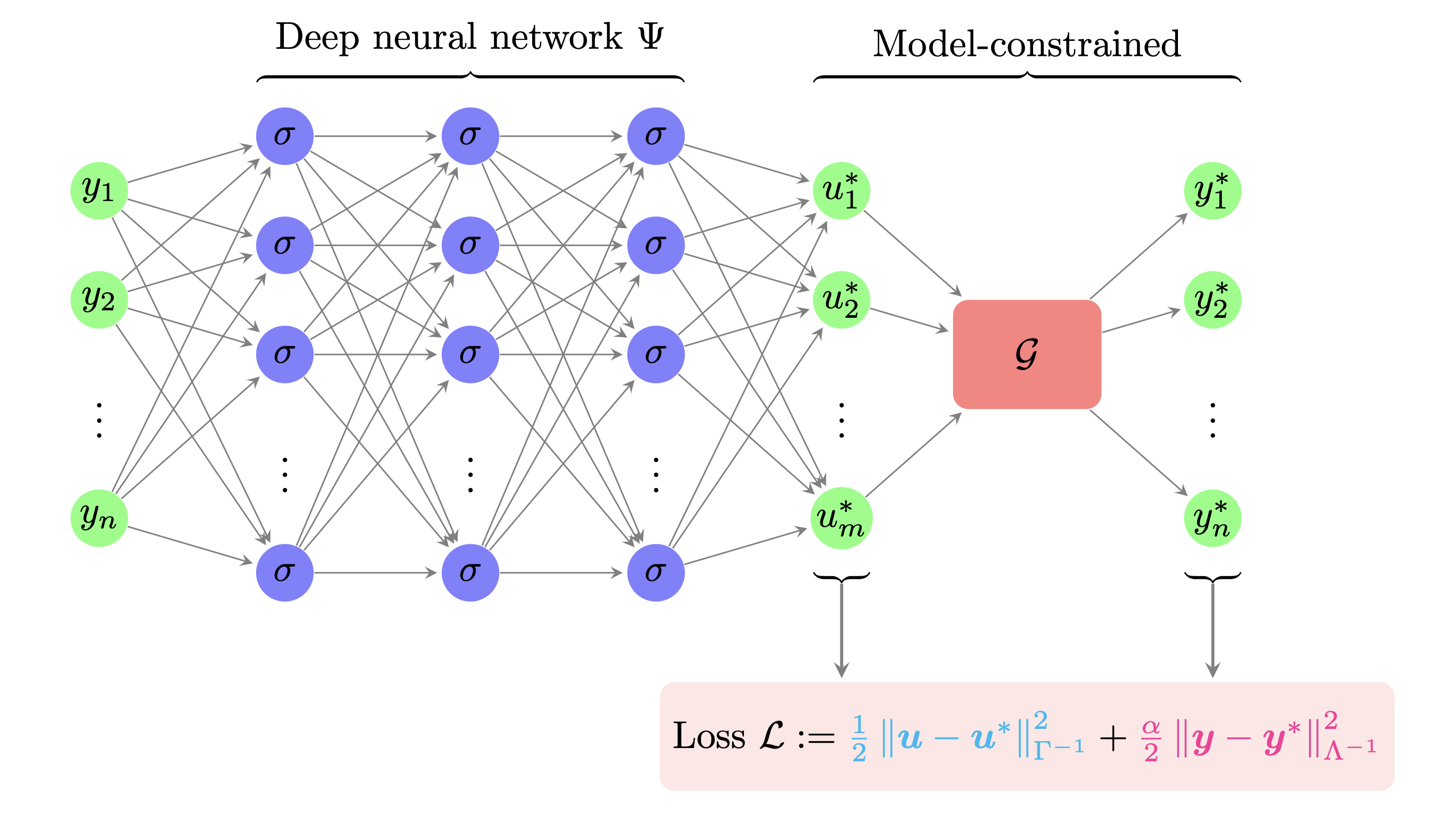 Figure 1: Model-constrained neural network architecture mcDNN. The observables y is fed into the neural network Ψ. The parameter u∗ predicted by the netork is pushed through the PtO map G to generate the corresponding predicted observations y∗. Both predicted parameters and observations are compared with ground truth u and y, respectively, to provide the mean-square error in the loss function L..
Significant Results
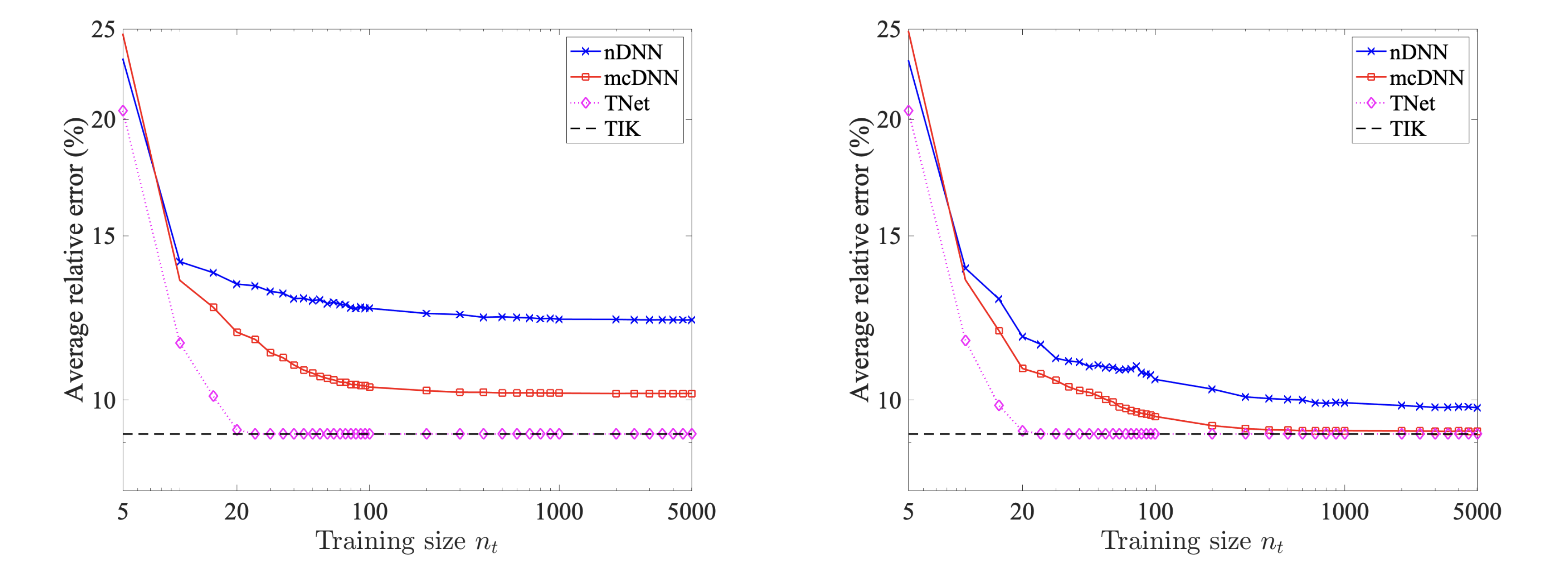 Figure 2: 1D Linear deconvolution problem The average relative error at the optimal regularization parameter versus the training size for nDNN, mcDNN, TNet, and Tikhonov methods. The result for Case II (data augmentation technique) is on the left figure for training size up to $5000$, and a similar result is shown on the right figure for Case III (all distinct samples data).
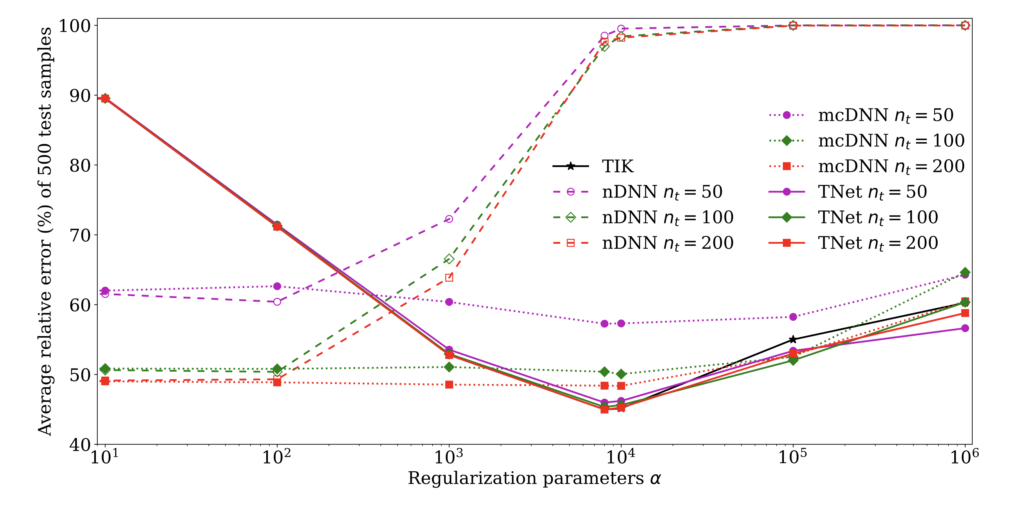 Figure 3: 2D heat conductivity inverse problem The average relative error over 500 test samples. The comparisons are done for nDNN (dashed curves), mcDNN (dotted curves), TNet (colored solids curves), and Tikhonov (TIK: black curve) over a wide range of regularization parameter values.
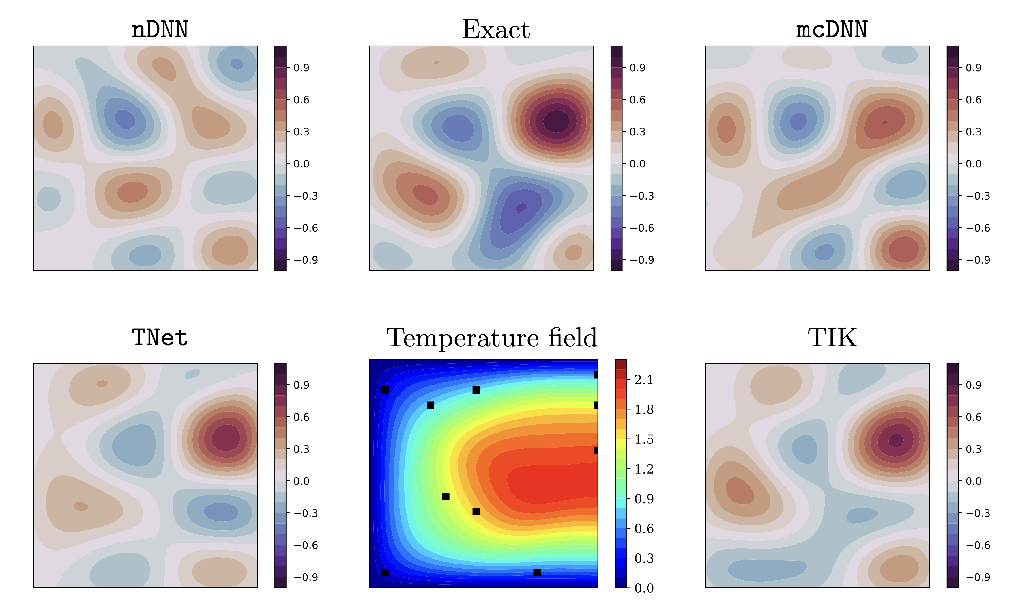 Figure 4: 2D heat conductivity inverse problem Predicted (reconstructed) heat conductivities for an unseen noisy test sample obtained by nDNN, mcDNN, and TNet neural networks along with the Tikhonov reconstruction. Shown in the middle column are the synthetic ground truth (Exact) conductivity and the corresponding temperature field for reference.
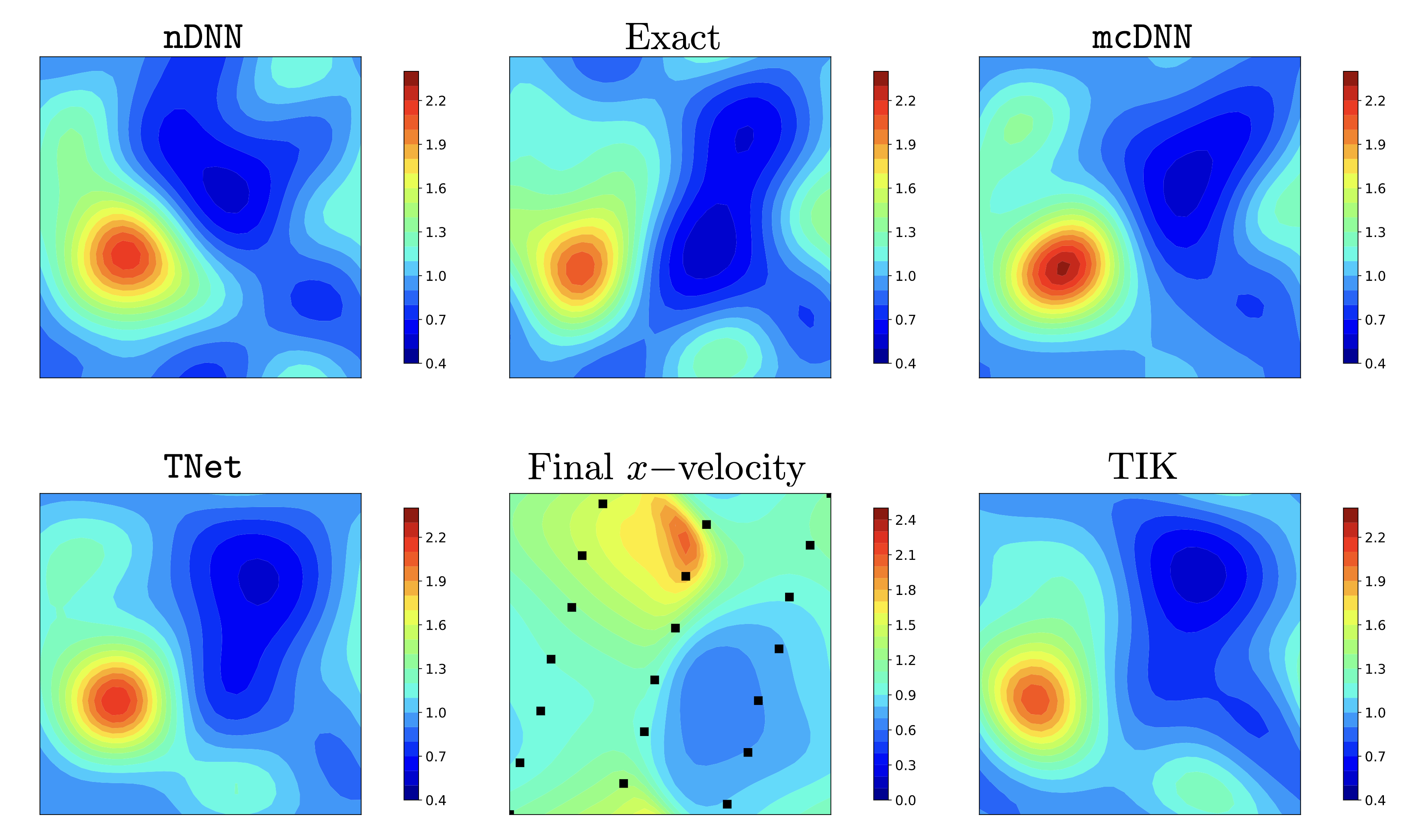 Figure 5: 2D Burger's equations. Predicted (reconstructed) initial x-velocity component for an unseen noisy test sample obtained by nDNN, mcDNN, and TNet neural networks along with the Tikhonov reconstruction. Shown in the middle column are the synthetic ground truth (Exact) x-velocity and the corresponding x-velocity at the final time for reference.
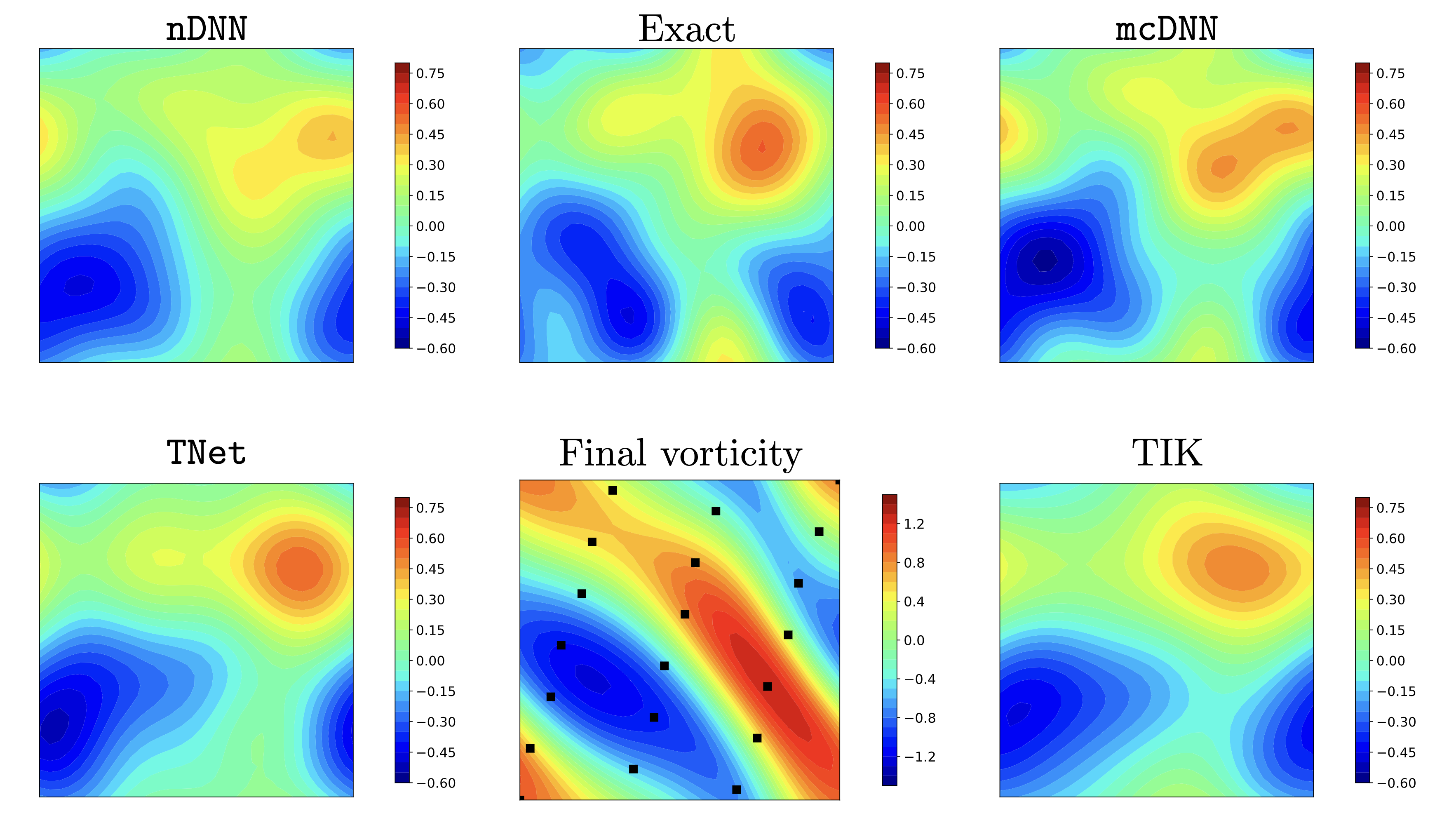 Figure 6: 2D Navier-Stokes equation Predicted (reconstructed) initial vorticities for an unseen noisy test sample obtained by nDNN, mcDNN, and TNet neural networks along with the Tikhonov reconstruction. Shown in the middle column are the synthetic ground truth (Exact) vorticity and the corresponding vorticity at the final time for reference.