Paper publication
Publication Link: https://www.sciencedirect.com/science/article/pii/S0045782525001847
Citation:
@article{van2025model,
  title={A model-constrained discontinuous Galerkin Network (DGNet) for compressible Euler equations with out-of-distribution generalization},
  author={Van Nguyen, Hai and Chen, Jau-Uei and Bui-Thanh, Tan},
  journal={Computer Methods in Applied Mechanics and Engineering},
  volume={440},
  pages={117912},
  year={2025},
  publisher={Elsevier}
}
Methodology
In this work, we developed a machine learning framework to solve shock-type PDEs, in particular, Compressible Euler equations. †he core idea is motivated by the dual mesh between Discontinuous Galerkin (DG) method and Graph Neural Network (GNN).
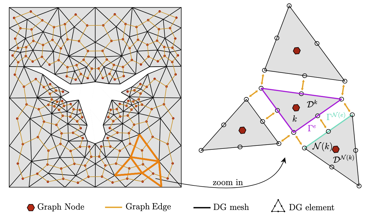 Figure 0: The dual mesh Discontinuous Galerkin (DG) method and Graph Neural Network (GNN) .
The training data flow is presented as shown in Figure 1. We integrate the data randomization and differentiable solvers to enhance the generalization of neural surrogate models.
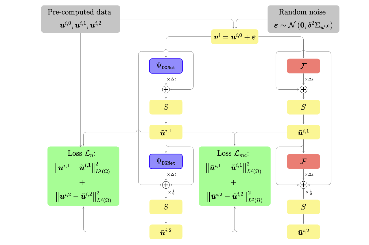 Figure 1: The schematic of DGNet network architecture.
Numerical results
- We work on 2D Euler equations
\[\begin{align*}
\frac{\partial \rho}{\partial t} + \frac{\partial (\rho u)}{\partial x} + \frac{\partial (\rho v)}{\partial y} &= 0 \\
\frac{\partial (\rho u)}{\partial t} + \frac{\partial (\rho u^2 + p)}{\partial x} + \frac{\partial (\rho u v)}{\partial y} &= 0 \\
\frac{\partial (\rho v)}{\partial t} + \frac{\partial (\rho u v)}{\partial x} + \frac{\partial (\rho v^2 + p)}{\partial y} &= 0 \\
\frac{\partial E}{\partial t} + \frac{\partial (u(E + p))}{\partial x} + \frac{\partial (v(E + p))}{\partial y} &= 0,
\end{align*}\]
where \(E\) is the total energy per unit volume:
\[E = \frac{p}{\gamma - 1} + \frac{\rho}{2}(u^2 + v^2)\]
Problem 1. Airfoil NACA0012
- Training data is generated from Airfoil AoA = 3 and Mach = 0.8, in time interval [0,1.2]s
- Test data is generated from Airfoil AoA = 3 and Mach = 0.8 and Airfoil AoA = 5 and Mach = 1.2 for time interval [0, 7.5]s
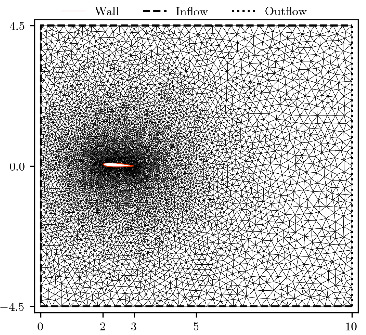 Figure 2: (Airfoil) Airfoil configuration AoA-3.
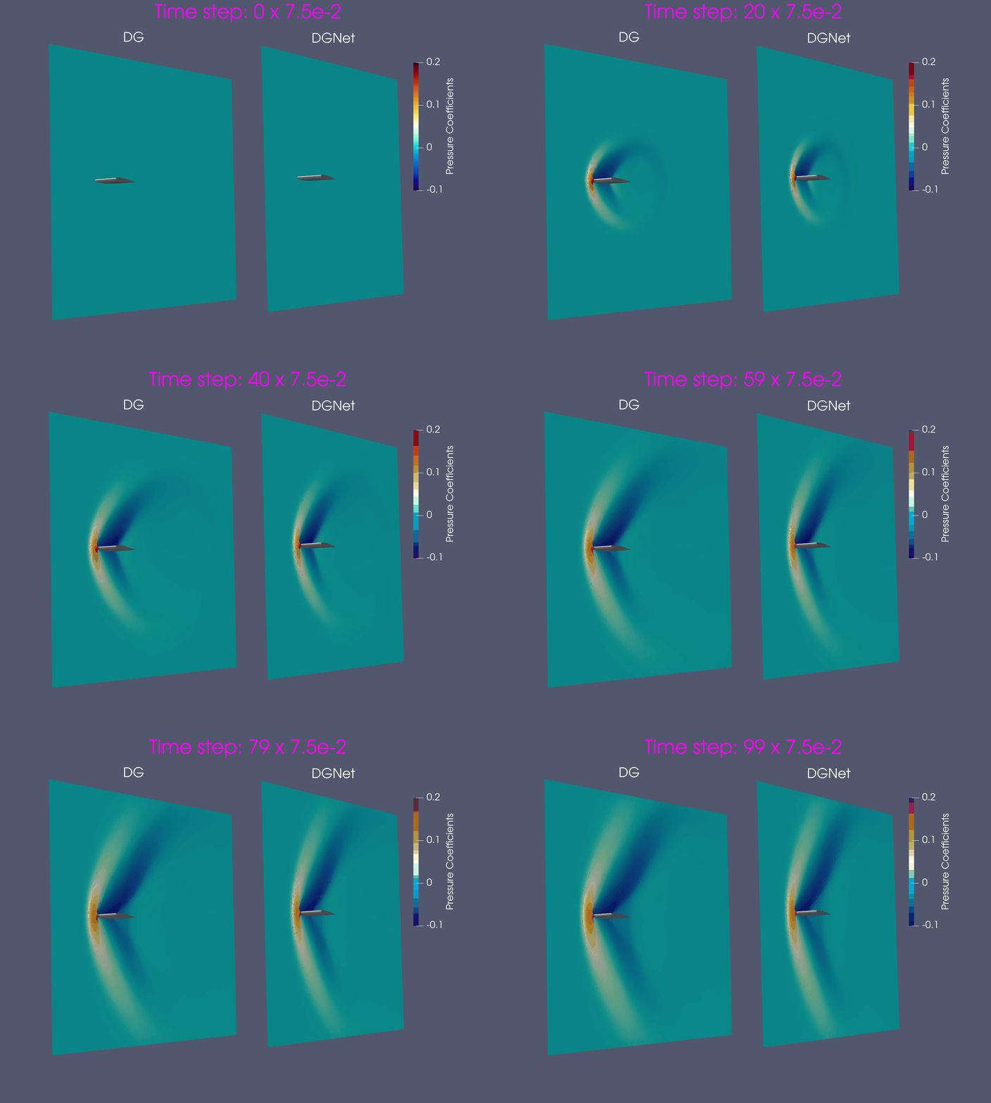 Figure 3: (Airfoil) predictions by DGNet for Airfoil NACA0012 of AoA = 5 and Mach = 1.2.
Problem 2. Euler configurations 6 & 12
- Training data is generated from Euler configuration 6 with time interval [0,0.16]s
- Test data is generated from Euler configuration 6 for time interval [0, 0.8]s and Euler configuration 12 for time interval [0, 0.25]s
 Figure 4: (Euler configurations) Information settings.
 Figure 5: (Euler configurations) predictions by DGNet for configuration 6.
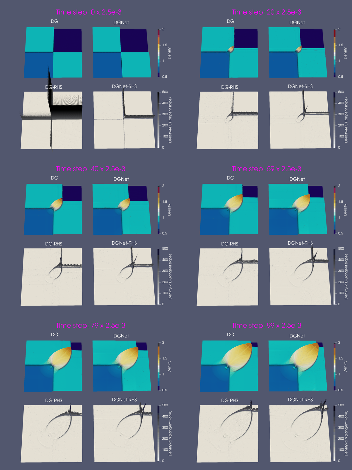 Figure 6: (Euler configurations) predictions by DGNet for configuration 12.
Problem 3: Double Mach Reflection
- Training data is generated with time interval [0,0.02]s
- Test data is generated with time interval [0, 0.25]s
 Figure 7: (Double Mach Reflection) model.
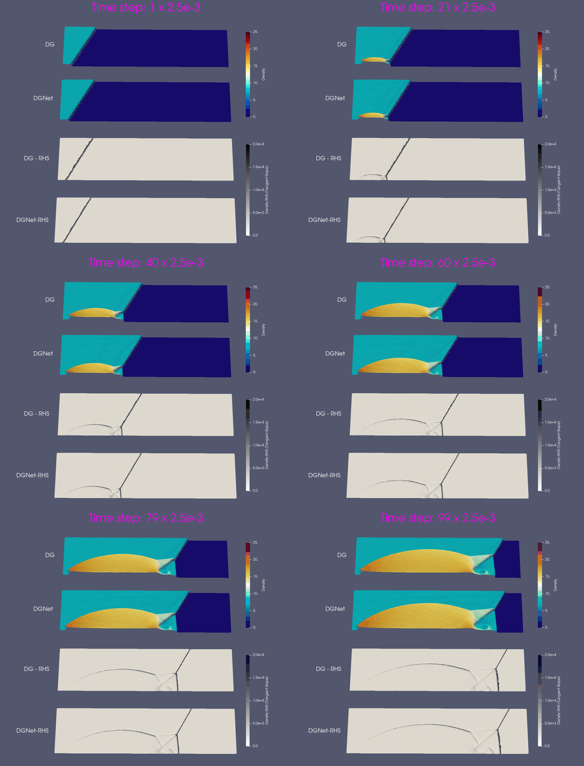 Figure 8: (Double Mach Reflection) predictions by DGNet.
Problem 4. Forward facing corner
- Training data is generated from Model 1 with time interval [0,1]s
- Test data is generated from Model 1 and Model 2 for time interval [0,4]s
 Figure 9: (Forward-facing corner) Model 1 and Model 2.
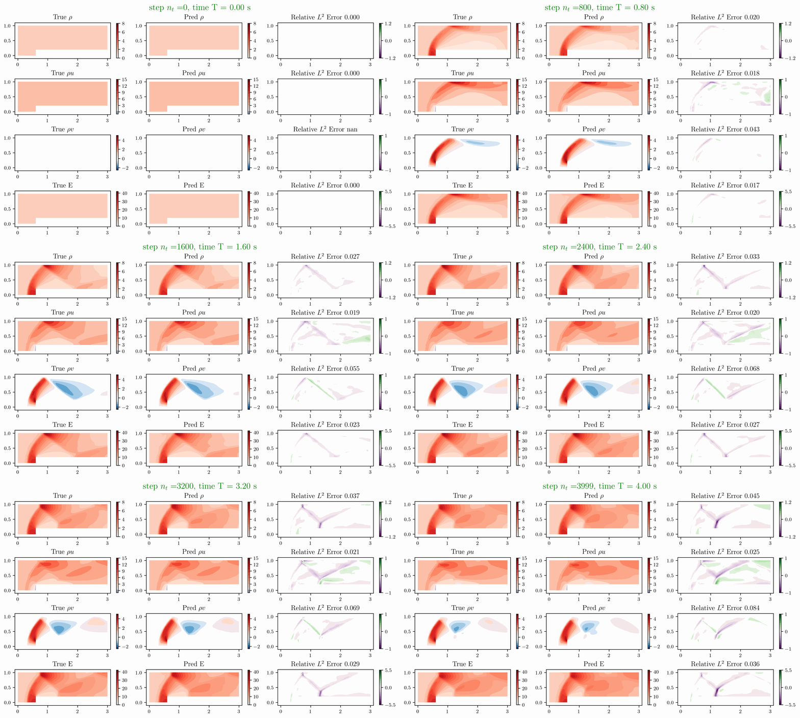 Figure 10: (Forward-facing corner) predictions by DGNet for Model 1.
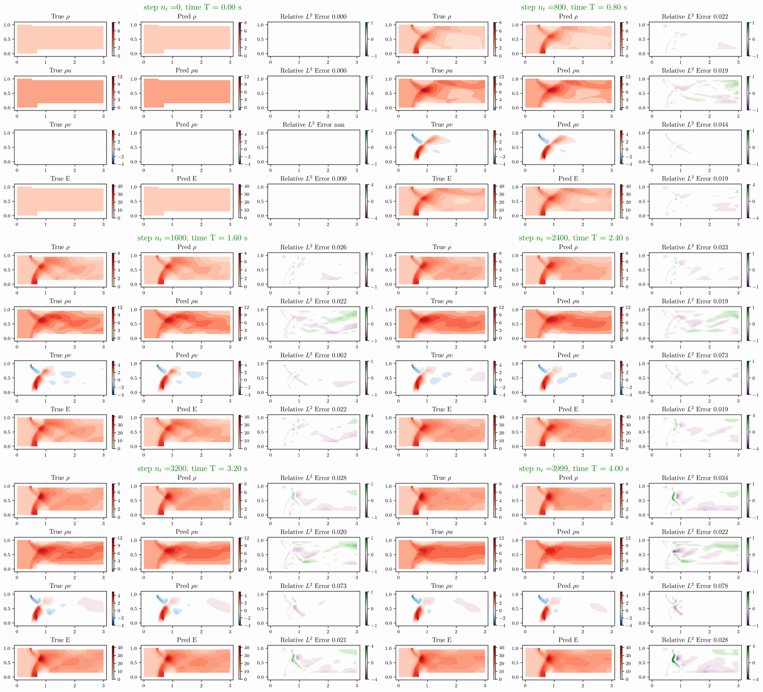 Figure 11: (Forward-facing corner) predictions by DGNet for Model 2.
Problem 5. ScramJet
- Training data is generated from Model 1 with time interval [0,1.6]s
- Test data is generated from Model 1 and Model 2 for time interval [0, 6]s
 Figure 12: (ScramJet) Model 1 and Model 2.
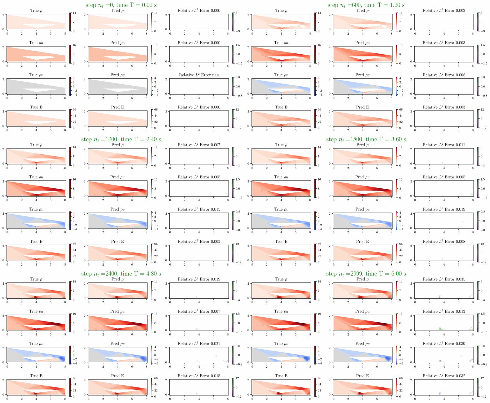 Figure 13: (ScramJet) predictions by DGNet for Model 1.
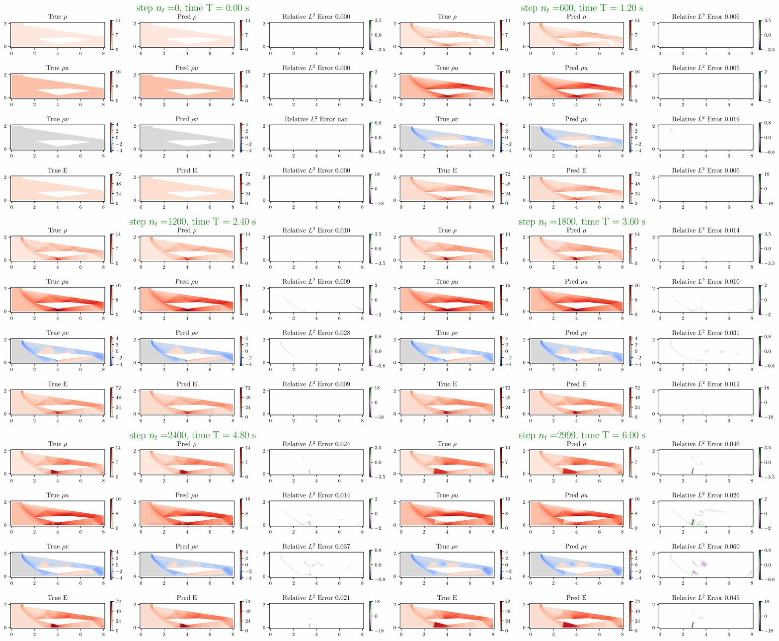 Figure 14: (ScramJet) predictions by DGNet for Model 2 .
Problem 6. Hypersonic flow over a sphere cone
- Training data is generated with time interval [0,3e-4]s
- Test data is generated with time interval [0, 1.5e-3]s
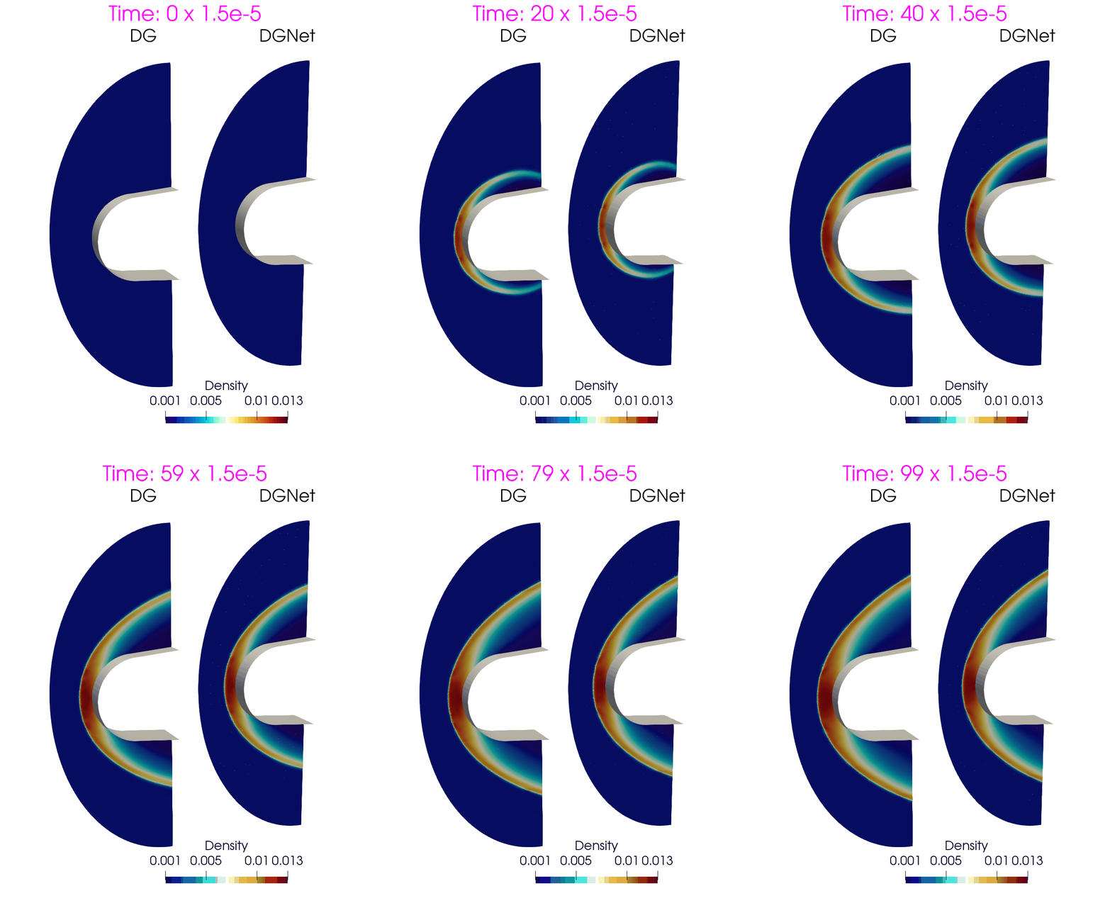 Figure 15: (Hypersonic flow) predictions by DGNet.